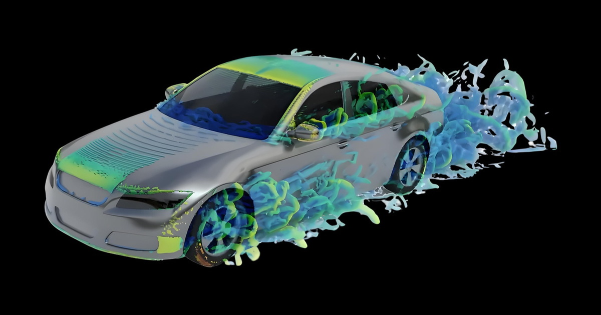
Turbulence is everywhere around us, visible to anyone who looks for it, and still unsolved. It is not only responsible for bumpy airplane rides. It is a first-order challenge for anyone designing and building things: cooling microprocessors, automotive aerodynamics and combustion engines, nuclear reactors, marine vessels, shipbuilding, and manufacturing. Ever since Leonardo da Vinci's first observations, we have had major gaps in our understanding of how turbulence works.
When I meet God, I am going to ask him two questions: Why relativity? And why turbulence? I really believe he will have an answer for the first.
Attributed to Horace Lamb
Turbulence, drag, and the growing demand for high-fidelity CFD
The stakes for simulating turbulence correctly are enormous. Roughly 30% of worldwide energy consumption is used to overcome drag in transportation, with turbulence as the primary cause.[1]
Engineers who understand turbulence better can manipulate it better, whether they are designing cars, buildings, or airplanes. The payoff is a meaningful cut in global CO₂ emissions,[1] and less fuel burned means more profit for a company.
The governing equations of fluid flow, the Navier-Stokes equations, have analytical solutions for only a handful of simple cases. For everything else, the approach is what it has been for decades: simulation. Discretize them and solve them numerically, and you get computational fluid dynamics (CFD), which models aerodynamic fields as they actually behave, turbulence and all, along with the mechanical deformation, heat transfer, and vibration that come with them. How closely the answer matches reality depends on the mesh, the numerical methods, and the physical models chosen.
In the absence of a solution, original equipment manufacturers (OEMs) run larger, more detailed simulations to get more accurate answers. The computational demand climbs with them.
Convergent Science and CoreWeave teamed up to run CONVERGE CFD software on high-performance infrastructure. The project had two aims: validate the accuracy of the GPU solver against a well-established test case, and measure how it scales across two very different classes of hardware: NVIDIA RTX PRO 6000 NVIDIA Blackwell Server Edition and NVIDIA HGX B200. We picked the highest-fidelity approach available, direct numerical simulation (DNS), and ran large jobs at increasing scale. Scale here means what the industry means by it: bigger cases. Case size is measured in cells, each one storing the aerodynamic variables the solver calculates.
Direct Numerical Simulation (DNS): the most accurate simulation there is
The industry workhorse is not DNS. It is Reynolds-Averaged Navier-Stokes (RANS), which trades some fidelity for a computational load you can actually afford. Turbulence happens at every scale at once, and computing all of it exactly is out of reach, so engineers add a turbulence model that computes the large motions and estimates the small ones. It works, and it's what the industry runs on. It also means the answer carries an anticipated level of acceptable error.
DNS removes the model (the equations we manufacture to close the system of partial differential equations, making it solvable). Every scale is computed directly with nothing left to approximate. It's the highest-fidelity simulation possible to humans and the reference against which every production turbulence model was calibrated.
The cost is resolution: resolving the smallest eddies means very small cells, and small cells force very short time steps. The work multiplies from both directions with respect to spatial and temporal resolution.
The high fidelity makes the computational load heavy, and the usual answer is to spread it across more GPUs. Each GPU then holds one chunk of the domain and needs its neighbors’ edge values before every time step, thousands of times over, with every GPU waiting on the slowest. Adding GPUs shrinks the work each one does and increases the communication between them, a trade-off we return to below. Because each step is short, that communication is no rounding error: it is a large share of the total, and a slow interconnect shows up immediately. Memory decides whether the case can run at all, before speed enters the conversation.
Which is why we chose DNS. If a cluster holds up under the hardest workload in CFD, the everyday cases that ask less of it have room to spare.
Strong vs weak scaling: what adding GPUs actually buys you
Adding GPUs to a simulation solves one of two problems, and it's worth being clear which one. Take simulating airflow over a car:
- Strong scaling: the same answer, sooner. Keep the mesh exactly as it is and add GPUs to finish faster. A job that took eight hours might now take three. The total job stays fixed; each GPU's share shrinks. Ideally, it would be double the GPUs, half the time (but it heavily depends on the problem).
- Weak scaling: the answer gets more accurate while the GPU resources increase to run it faster, at the same time. Double the resolution of the mesh, which makes the answer more accurate, and double the GPUs to satisfy the higher computational demand. An ideal case would be twice the size and take no longer than the smaller one did.

Computational demand keeps climbing because OEMs want larger and more detailed cases, not faster versions of the ones they can already run. So weak scaling is the number we lead with, and strong scaling serves as the check for how much speed you can buy for a case you already have.
Table 1 below summarizes the runs in the test matrix. Every run uses the same well-validated classical case, turbulent flow losing energy with time in a three-dimensional rectangular space.
Scale factor is relative to the base case of ~16.8 M cells
Outside the scaling matrix, we set out to find the largest case this configuration and hardware could carry. We extended the 512³ case four times in a single direction to 536 million cells and ran it on two NVIDIA HGX B200 instances, 16 NVIDIA Blackwell GPUs. It ran to completion in 3.62¹ hours.
It isn't part of the scaling study because it answers how far the system goes, not how efficiently the system scaled. DNS carries fewer equations than the RANS models industry runs every day, so expect a production case at the same cell count to need more memory.
Intranode vs. internode scaling: why benchmark numbers aren't comparable
There's a second distinction that matters just as much and gets labeled far less often: where the GPUs are.
- Intranode (within a node): all the GPUs inside one server. They talk to each other over the machine's internal connections: PCIe on RTX PRO Server, or NVIDIA NVLink™ on NVIDIA HGX B200, which is considerably faster.
- Internode (between nodes): GPUs spread across multiple servers. They talk over the network fabric between machines. In our case, that is 400 Gb/s leveraging NVIDIA Quantum-2 InfiniBand networking.
This is why scaling numbers are so often incomparable. “We added GPUs and measured the scaling” describes two very different experiments, and which one you ran changes what the number measures: the memory on each GPU, the link between GPUs inside a server, or the fabric between servers. We come back to each below.
How to size a GPU CFD job: memory first, FLOPS second
Anyone procuring GPU capacity for simulation work learns this early on, and often learns it the hard way: Memory decides whether your case runs at all. FLOPS only decide how fast.
The cell count tells you how big the job is. It doesn't tell you how much memory it needs. That depends on what each cell has to hold.
- What physics you've turned on: Every cell stores a set of numbers, and each effect you model adds more. A combustion case tracking chemical reactions stores a value for every chemical species in every cell, which can run to dozens or hundreds. Plain airflow stores a handful. A turbulence model adds its own transport equations and variables; DNS removes them, then takes far more back by requiring a much finer mesh.
- How precisely those numbers are stored: double precision instead of single doubles every one of them.
- What the solver keeps on hand: some methods hold several snapshots of the flow field at once, plus working space for the math, on top of the answer itself.
- Whether the mesh changes as it progresses: CONVERGE’s Adaptive Mesh Refinement concentrates cells where the physics needs them and removes them elsewhere, which keeps the overall count lower than a uniformly fine mesh would. It also means the count varies over a run, so size against the peak cell count rather than the starting mesh.
What we ran sits at the lean end of that list — DNS, single-phase, no reactions. A production case with the same cell count but more physics will need more memory per cell, so any rule of thumb drawn from these numbers will underestimate what your own case requires.
NVIDIA RTX PRO 6000 Blackwell Server Edition vs. NVIDIA HGX B200: which hardware for which CFD problem?
Industrial CFD lives in two regimes: the case that fits inside a single server, which is much of everyday work, and the case that doesn't, which is where the frontier is. A single GPU SKU cannot reasonably characterize both of those regimes, which is why we ran the same validated case on two very different classes of hardware.
Every row in that table answers a single question: how much communication between GPUs does your case require?
If your case fits inside a single node, NVIDIA RTX PRO Server covers it. Much everyday industrial simulation lives here, and inside one box, the boundary exchanges never leave the chassis, so PCIe carries them. That is the regime it is built for.
When a case has to span nodes, NVIDIA HGX B200 is what carries it. Nearly twice the memory per GPU means fewer GPUs and fewer boundaries to coordinate across. Close to five times the memory bandwidth matters for a solver whose inner loop is bound by moving data rather than arithmetic. NVLink handles traffic that stays inside the node, and non-blocking NVIDIA Quantum InfiniBand carries traffic that leaves it. Together they set the clock: five eddy turnover times, a standard measure of simulated physical time, in 3.62 hours.
This was one of the best clusters we've tested CONVERGE on. The CoreWeave team took the time to understand our workload and what we were trying to prove, then built the environment around it, and the results showed it. We pushed further than we expected and the scaling held up.
Cooper Burns, HPC Team Lead at Convergent Science
Convergent Science has published the full study: validation against published DNS data, weak and strong scaling on both GPUs, and their analysis of what currently limits efficiency in a double-precision solver.
NVIDIA GPUDirect RDMA, non-blocking NVIDIA Quantum InfiniBand, and topology you can act on
The table above names the technologies. What follows is what they do once a solver is running, and why together they decide the shape of a scaling curve.
Every scaling number is a measurement of coordination overhead. The arithmetic inside each block parallelizes cleanly, with every GPU crunching its own share. What costs you is the handoff at the boundaries, every timestep, with every GPU waiting on the slowest.
Three things decide what that costs:
- NVLink inside the node: moves boundary data between GPUs in the same chassis at a rate PCIe cannot match.
- NVIDIA GPUDirect™ GPUDirect RDMA (remote direct memory access) between nodes: data moves straight from one GPU's memory into another's, with no staging through host memory and no CPU in the path. For a solver that synchronizes every timestep, a host-memory round trip stops being marginal overhead and becomes the dominant cost.
- A non-blocking fabric you can see into: an oversubscribed network means a 16-GPU run is only as fast as its worst-placed GPU. Ours is 400 Gb/s non-blocking — every node can reach every other at full speed at once. But capacity is not the point. Scaling only holds if GPU placement matches the physical topology, and on a generic cloud endpoint, topology is hidden. When a curve sags, you cannot see why, so you cannot fix it. Here, it is visible and actionable in workload placement, which is the difference between a benchmark and a system you can debug.
The whole study ran through SUNK (CoreWeave's implementation of Slurm on Kubernetes) on bare-metal nodes, so Convergent Science's team submitted jobs the way they always have.
Bring us your simulation
Whatever solver you run and however large the case, tell us what you are trying to simulate and we will tell you what it takes to run it. We have taken DNS to half a billion cells on two nodes, and we know where the curves sag and why.
Schedule a call
Keep reading:
- Wayve, Decart, NEURA Robotics, Nissan: all running physical AI on CoreWeave
- Explore CoreWeave’s physical AI stack